gganimate is an extension of the grammar of graphics, as implemented by the ggplot2 package, that adds support for declaring animations using an API familiar to users of ggplot2.
The following introduction assumes familiarity with ggplot2 to the extent that constructing static plots and reading standard ggplot2 code feels natural. If you are new to both ggplot2 and gganimate you’ll benefit from exploring the trove of ggplot2 documentation, tutorials, and courses available online first (see the ggplot2 webpage for some pointers).
Your First Animation
We’ll jump right into our first animation. Don’t worry too much about understanding the code, as we’ll dissect it later.
library(gganimate)
#> Loading required package: ggplot2

# We'll start with a static plot
p <- ggplot(iris, aes(x = Petal.Width, y = Petal.Length)) +
  geom_point()

plot(p)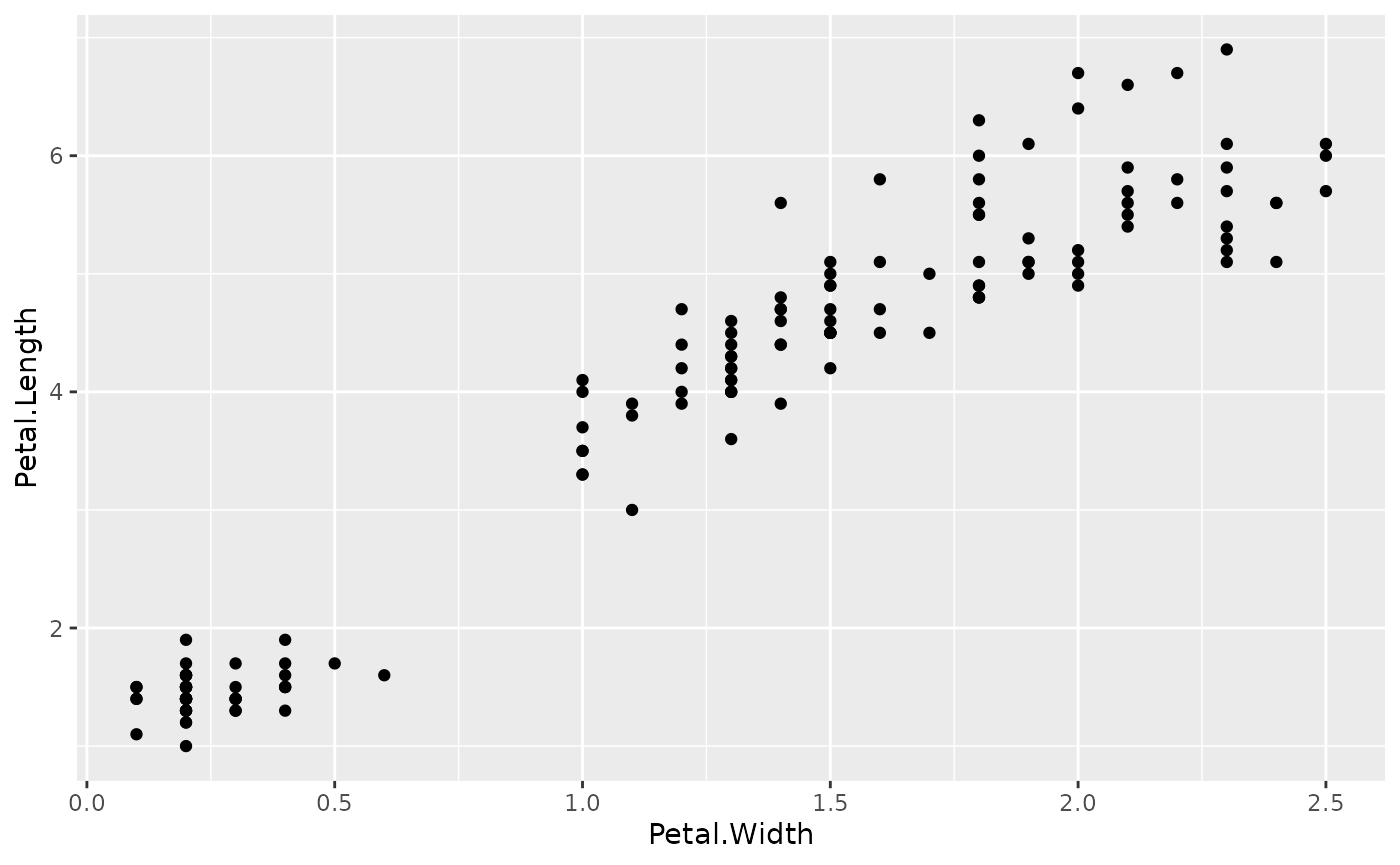
You go from a static plot made with ggplot2 to an animated one, simply by adding on functions from gganimate.
anim <- p +
  transition_states(Species,
                    transition_length = 2,
                    state_length = 1)

anim
❗
transition_states()splits up plot data by a discrete variable and animates between the different states.
As can be seen, very few additions to the plot results in a quite
complex animation. So what did we do to get this animation? We added a
type of transition. Transitions are functions that interpret
the plot data in order to somehow distribute it over a number of frames.
transition_states() specifically splits the data into
subsets based on a variable in the data (here Species), and
calculates intermediary data states that ensures a smooth transition
between the states (something referred to as tweening).
gganimate provides a range of different transitions, but for
the rest of the examples we’ll be sticking to
transition_states() and see how we can modify the
output.
Easing
When transition_states() calculates intermediary data
for the tweening, it needs to decide how the change from one value to
another should progress. This is a concept called easing. The
default easing is linear, but others can be used, potentially
only targeting specific aesthetics. Setting easing is done with the
ease_aes() function. The first argument sets the default
easing and subsequent named arguments sets it for specific
aesthetics.
anim +
  ease_aes('cubic-in-out') # Slow start and end for a smoother look
❗
ease_aes()defines the velocity with which aesthetics change during an animation.
anim +
  ease_aes(y = 'bounce-out') # Sets special ease for y aesthetic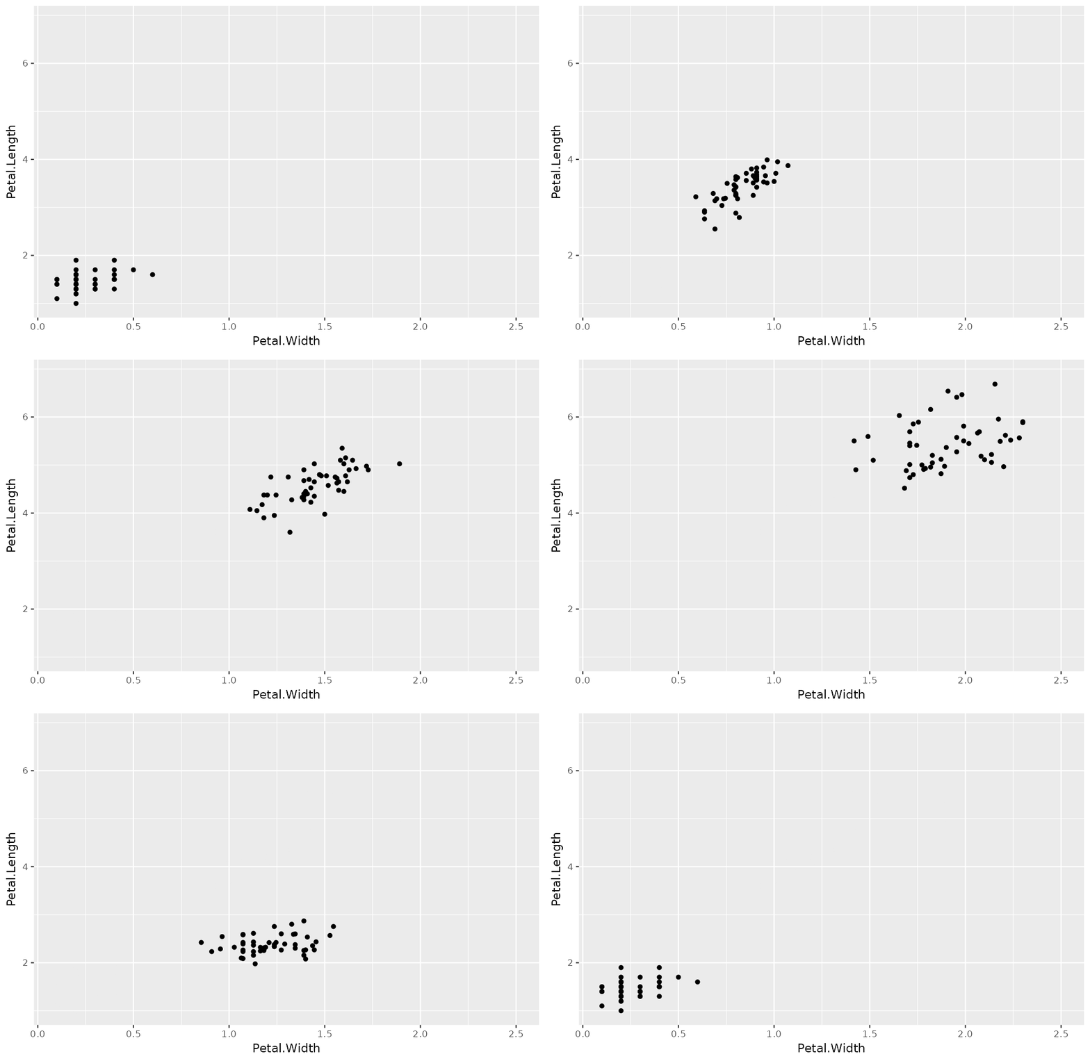
Labeling
It can be quite hard to understand an animation without any indication as to what each time point relates to. gganimate solves this by providing a set of variables for each frame, which can be inserted into plot labels using glue syntax.
anim +
  ggtitle('Now showing {closest_state}',
          subtitle = 'Frame {frame} of {nframes}')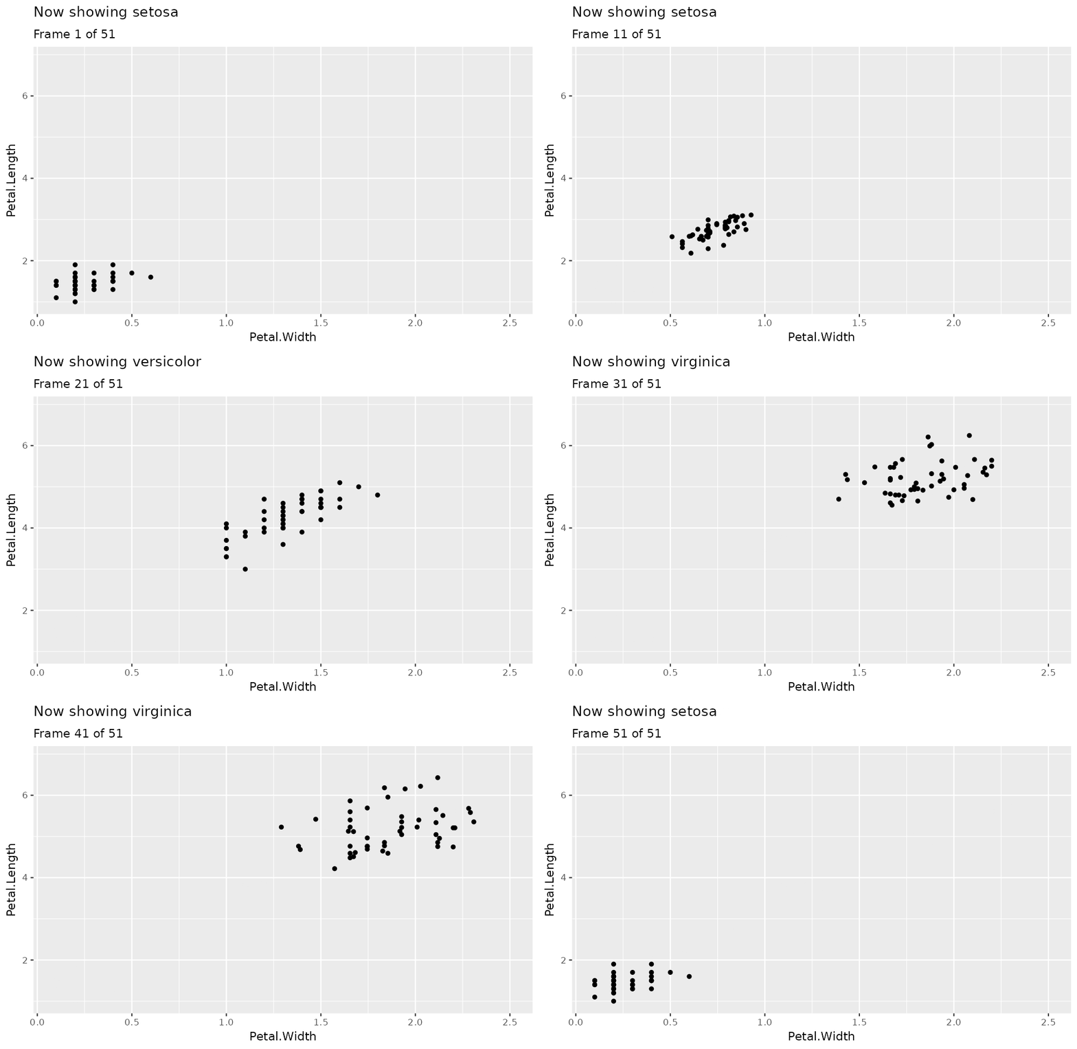
❗ Use glue syntax to insert frame variables in plot labels and titles.
Different transitions provide different frame variables.
closest_state only makes sense for
transition_states() and is thus only available when that
transition is used.
Object Permanence
In the animation above, it appears as if data in a single measurement changes gradually as the flower being measured on somehow morphs between three different iris species. This is probably not how Fisher conducted the experiment and got those numbers. In general, when you make an animation, graphic elements should only transition between instances of the same underlying phenomenon. This sounds complicated but it is more or less the same principle that governs makes sense to draw a line between two observations. You wouldn’t connect observations from different iris species, but repeated observations on the same plant would be fine to connect. Same thing with animations.
Just to make this very clear (it is an important concept). The line plot equivalent of our animation above is:
ggplot(iris, aes(x = Petal.Width, y = Petal.Length)) +
  geom_line(aes(group = rep(1:50, 3)), colour = 'grey') +
  geom_point()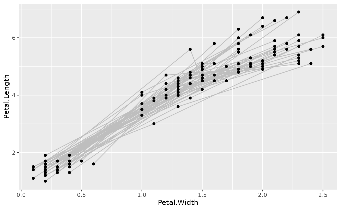
Ugh…
So, how do we fix this and tell gganimate to not morph
observations from different species into each others? The key is the
group aesthetic. You may be familiar with this aesthetic from
plotting lines and polygons, but in gganimate it takes a more
central place. Data that have the same group aesthetic are interpreted
as being linked across states. The semantics of the group aesthetic in
ggplot2 is such that if it is undefined it will get calculated
based on the interaction of all discrete aesthetics (sans
label). If none exists, such as in our iris animation, all
data will get the same group, and will thus be matched by
gganimate. So, there are two ways to fix our plot:
- Add some aesthetics that distinguish the different species
ggplot(iris, aes(x = Petal.Width, y = Petal.Length)) +
  geom_point(aes(colour = Species)) +
  transition_states(Species,
                    transition_length = 2,
                    state_length = 1)
- Set the group directly
ggplot(iris, aes(x = Petal.Width, y = Petal.Length)) +
  geom_point(aes(group = seq_along(Species))) +
  transition_states(Species,
                    transition_length = 2,
                    state_length = 1)
❗ The group aesthetic defines how the data in a layer is matched across the animation.
In general 2) is preferred as it makes the intent explicit. It also makes it possible to match data with different discrete aesthetics such as keeping our (now obviously faulty) transition while having different colour for the different species)
ggplot(iris, aes(x = Petal.Width, y = Petal.Length)) +
  geom_point(aes(colour = Species, group = 1L)) +
  transition_states(Species,
                    transition_length = 2,
                    state_length = 1)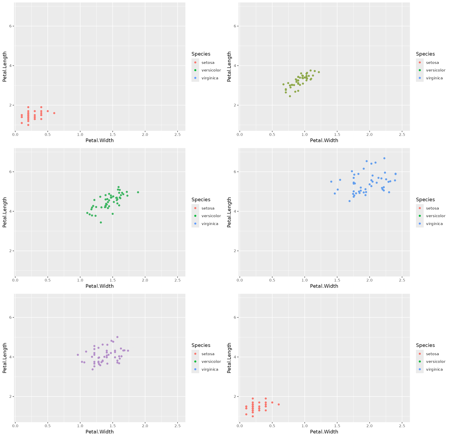
Enter and Exit
While we may have made our animation more correct by separating the data from the different species, we have also made it quite a bit more boring. Now it simply appears as three static plots shown one at a time, which is hardly an attention grabber. If only there were a way to animate the appearance and disappearance of data…
Enter the enter and exit functions. These
functions are responsible for modifying the state of appearing
(entering) and disappearing (exiting) data, so that the animation can
tween from and to the new state. Let’s spice up our animation a bit:
anim <- ggplot(iris, aes(x = Petal.Width, y = Petal.Length)) +
  geom_point(aes(colour = Species), size = 2) +
  transition_states(Species,
                    transition_length = 2,
                    state_length = 1)

anim +
  enter_fade() +
  exit_shrink()
❗
enterandexitfunctions are used to modify the aesthetics of appearing and disappearing data so that their entrance or exit may be animated.
gganimate comes with a range of different functions, and
using the enter_manual() and exit_manual()
functions you can create your own. Enter and exit functions are
composable though, so you can often come pretty far by combining
preexisting ones
anim +
  enter_fade() + enter_drift(x_mod = -1) +
  exit_shrink() + exit_drift(x_mod = 5)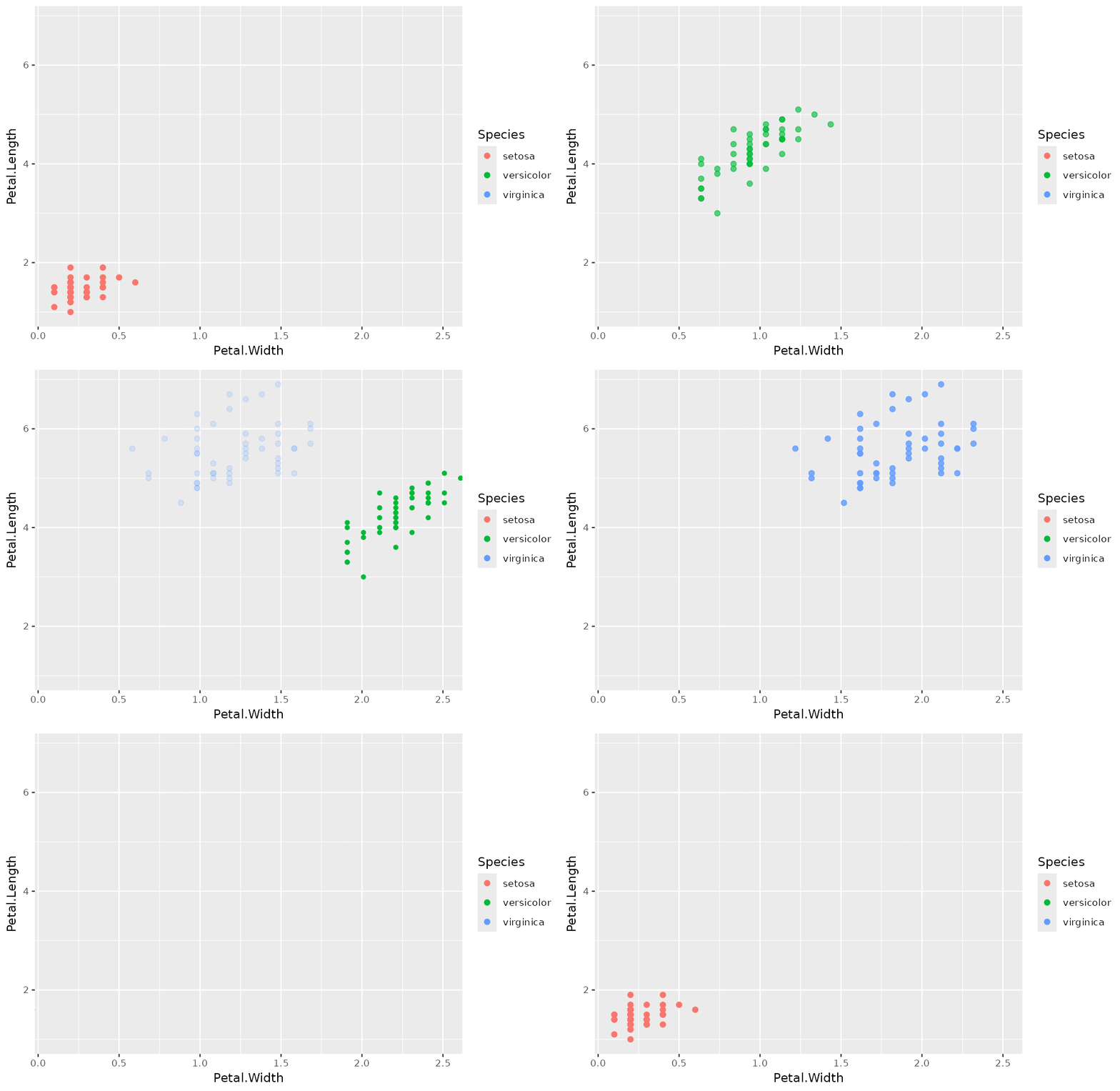
Rendering
In the examples above the animations has simply appeared when we printed the animation object, just like we would expect from ggplot2. As a lot of things are happening automatically, and you might want to take control, this section will give a brief overview of the rendering.
gganimate’s model for an animation is dimensionless in the
same way as ggplot2 describe plots independent of the final
width and height of the plot. This means that the final number of frames
and its frame-rate are only ever given when you ask gganimate
to render the animation. When you print an animation object the
animate() function is called on the animation with default
arguments, some of which are:
-
nframes sets the number of frames to render
(defaults to
100) -
fps sets the frame rate of the animation in
frames/sec (defaults to
10) -
dev sets the device used to render each frame
(defaults to
'png') -
renderer sets the function used to combine each
frame into an animate (defaults to
gifski_renderer())
There are other arguments as well (e.g. ... will be
passed on to the device so you can set width, height, dpi, etc), but
these are the most important. If you don’t like the defaults you can
either call animate() directly with values of your
choosing, or modify the defaults by setting new with
options(gganimate.<argument> = <value>).
A topic that requires some additional words are the renderers. The
default will use gifski
to combine the frames into a gif. gifs are great because they are
virtually supported everywhere, and gifski is both a very fast, and very
high quality converter. Still, you may have reasons to want a different
output. gganimate is quite agnostic to how you want to combine
the frames and, while it comes with a set of predefined renderers, any
function that takes a vector of paths to image files along with a
frame-rate, will do. The return value of your renderer is what is
ultimately returned by the animate() function.
Below are a couple of examples of different animate()
calls:
# Video output
animate(
  anim + enter_fade() + exit_fly(y_loc = 1),
  renderer = av_renderer()
)
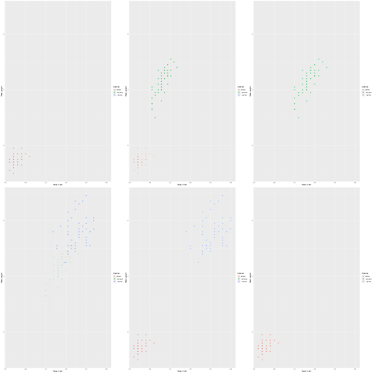
# Different size and resolution
animate(
  anim + ease_aes(x = 'bounce-out') + enter_fly(x_loc = -1) + exit_fade(),
  width = 400, height = 600, res = 35
)
If you need to save the animation for later use you can use the
anim_save() function. It works much like
ggsave() from ggplot2 and automatically grabs the
last rendered animation if you do not specify one directly.
Want more?
This guide is far from exhaustive, but have hopefully given you a broad understanding of how gganimate works. There are still more to explore as we have only scratched the surface of transitions, let alone mentioned views and shadows. But for now this is left to you. There is a fantastic joy in discovery and with the things you have now learned you are ready to go digging on your own.